Gene Set Enrichment Analysis with NMFscape
NMFscape Development Team
2025-09-12
Source:vignettes/go-enrichment.Rmd
go-enrichment.RmdIntroduction
Gene set enrichment analysis is a powerful approach to interpret the biological meaning of gene expression programs identified by Non-negative Matrix Factorization (NMF). This vignette demonstrates how to perform and visualize Gene Ontology (GO) enrichment analysis using NMFscape’s integrated workflow.
We’ll use the Zeisel brain dataset, which contains diverse brain cell types with distinct molecular signatures - perfect for demonstrating how NMF programs capture biologically meaningful gene expression patterns.
Setup and Data Preparation
library(NMFscape)
library(scRNAseq)
library(scuttle)
library(scater)
library(scran)
library(ggplot2)
library(patchwork)

# For GO enrichment (install if needed)
# BiocManager::install(c("clusterProfiler", "org.Mm.eg.db"))
library(clusterProfiler)
library(org.Mm.eg.db)
Load and Process Brain Data
# Load the Zeisel mouse brain dataset
sce <- ZeiselBrainData()

cat("Original dataset:", nrow(sce), "genes,", ncol(sce), "cells\n")
#> Original dataset: 20006 genes, 3005 cells
cat("Brain cell types:", length(unique(sce$level1class)), "major classes\n")
#> Brain cell types: 7 major classes

# Show the brain cell type distribution
table(sce$level1class)
#>
#> astrocytes_ependymal    endothelial-mural         interneurons
#>                  224                  235                  290
#>            microglia     oligodendrocytes        pyramidal CA1
#>                   98                  820                  939
#>         pyramidal SS
#>                  399
# Quality control and preprocessing
sce <- addPerCellQCMetrics(sce)
sce <- addPerFeatureQCMetrics(sce)

# Filter for quality and computational efficiency
sce <- sce[rowData(sce)$detected >= 10, ]  # Keep genes detected in >=10 cells
sce <- sce[, colData(sce)$detected >= 500]  # Keep cells with >=500 detected genes

# Subset for faster analysis (optional)
set.seed(42)
if (ncol(sce) > 1200) {
  cell_subset <- sample(ncol(sce), 1200)
  sce <- sce[, cell_subset]
  cat("Randomly subsetted to 1200 cells for computational efficiency\n")
}
#> Randomly subsetted to 1200 cells for computational efficiency

# Normalize
sce <- logNormCounts(sce)

# Select highly variable genes for focused analysis
dec <- modelGeneVar(sce)
top_hvgs <- getTopHVGs(dec, n = 1000)  # Focus on top variable genes
sce <- sce[top_hvgs, ]

cat("Processed dataset:", nrow(sce), "genes,", ncol(sce), "cells\n")
#> Processed dataset: 1000 genes, 1200 cells
NMF Analysis
# Run NMF to identify gene expression programs
sce <- runNMFscape(sce, k = 8, verbose = FALSE)

# Add UMAP for visualization
sce <- runPCA(sce, ncomponents = 50)
sce <- runUMAP(sce, dimred = "PCA")

cat("NMF completed: identified", ncol(getBasis(sce)), "gene expression programs\n")
#> NMF completed: identified 8 gene expression programs
Let’s visualize the programs in UMAP space to see their spatial organization:
# Visualize programs in UMAP space
program_plots <- list()
for (i in 1:4) {  # Show first 4 programs
  program_plots[[i]] <- vizUMAP(sce, program = i,
                               title = paste("Program", i))
}

# Combine plots
(program_plots[[1]] + program_plots[[2]]) /
(program_plots[[3]] + program_plots[[4]])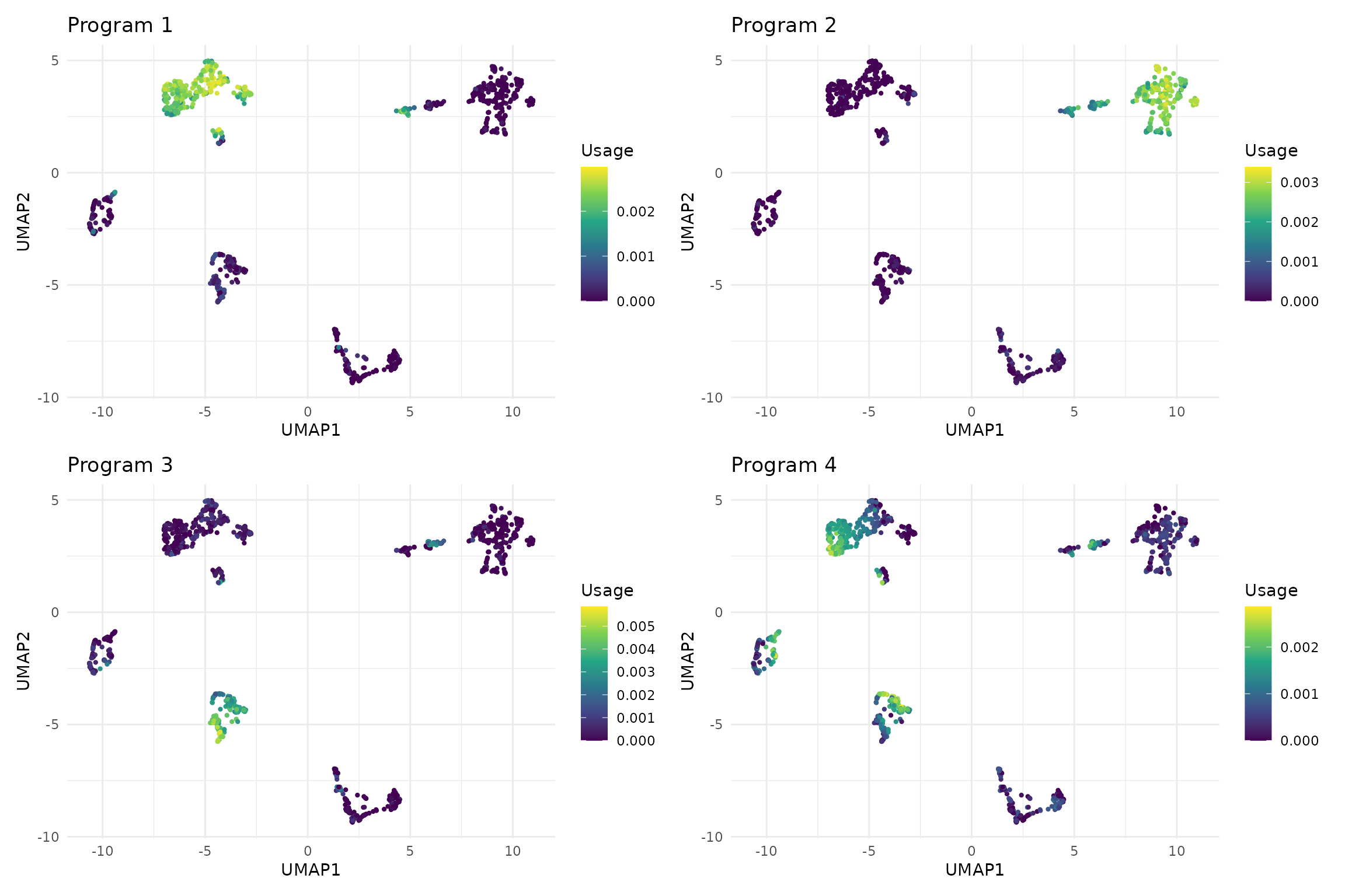
GO Enrichment Analysis
Now we’ll perform GO enrichment analysis to understand the biological functions associated with each gene expression program.
# Run GO enrichment analysis for all programs
cat("Running GO enrichment analysis...\n")
#> Running GO enrichment analysis...
go_results <- runProgramGOEnrichment(
  sce,
  organism = "mouse",      # Mouse brain data
  n_genes = 50,           # Use top 50 genes per program
  ont = "BP",             # Biological Process ontology
  pvalue_cutoff = 0.05    # Significance threshold
)
#> Detected gene ID type: SYMBOL
#> Running GO enrichment for NMF_2 ...
#>   Converted 1 genes to 1 Entrez IDs
#> Running GO enrichment for NMF_4 ...
#>   Converted 3 genes to 3 Entrez IDs
#> Running GO enrichment for NMF_6 ...
#>   Converted 6 genes to 6 Entrez IDs
#> Running GO enrichment for NMF_8 ...
#>   Converted 3 genes to 3 Entrez IDs
#> GO enrichment completed for 4 programs

# Summary of results
cat("GO Enrichment Results:\n")
#> GO Enrichment Results:
cat("Programs with significant GO terms:", length(go_results), "\n")
#> Programs with significant GO terms: 4

for (i in seq_along(go_results)) {
  program_name <- names(go_results)[i]
  n_terms <- nrow(go_results[[program_name]])
  cat("-", program_name, ":", n_terms, "significant GO terms\n")
}
#> - NMF_2 : 35 significant GO terms
#> - NMF_4 : 27 significant GO terms
#> - NMF_6 : 14 significant GO terms
#> - NMF_8 : 481 significant GO terms
Let’s examine the top GO terms for each program:
# Show top GO terms for each program
for (i in 1:min(4, length(go_results))) {
  program_name <- names(go_results)[i]
  go_result <- go_results[[program_name]]

  if (nrow(go_result) > 0) {
    cat("\n=== Top GO terms for", program_name, "===\n")

    # Convert to data.frame if needed and show top terms
    if (inherits(go_result, "enrichResult")) {
      go_df <- as.data.frame(go_result)
    } else {
      go_df <- go_result
    }

    top_terms <- head(go_df[, c("Description", "pvalue", "p.adjust", "Count")], 6)
    print(top_terms)
  }
}
#>
#> === Top GO terms for NMF_2 ===
#>                                                Description       pvalue
#> GO:0042759      long-chain fatty acid biosynthetic process 0.0009364595
#> GO:0035235 ionotropic glutamate receptor signaling pathway 0.0010405105
#> GO:0022010              central nervous system myelination 0.0011792453
#> GO:0032291     axon ensheathment in central nervous system 0.0011792453
#> GO:0014002                           astrocyte development 0.0013526637
#> GO:1990806      ligand-gated ion channel signaling pathway 0.0015607658
#>               p.adjust Count
#> GO:0042759 0.008800985     1
#> GO:0035235 0.008800985     1
#> GO:0022010 0.008800985     1
#> GO:0032291 0.008800985     1
#> GO:0014002 0.008800985     1
#> GO:1990806 0.008800985     1
#>
#> === Top GO terms for NMF_4 ===
#>                                     Description       pvalue     p.adjust Count
#> GO:0042255                    ribosome assembly 1.407687e-05 0.0003941523     2
#> GO:0022618         protein-RNA complex assembly 1.236573e-04 0.0012685784     2
#> GO:0071826     protein-RNA complex organization 1.359191e-04 0.0012685784     2
#> GO:0042254                  ribosome biogenesis 3.656976e-04 0.0025598830     2
#> GO:0140694      membraneless organelle assembly 6.807130e-04 0.0034275551     2
#> GO:0022613 ribonucleoprotein complex biogenesis 7.344761e-04 0.0034275551     2
#>
#> === Top GO terms for NMF_6 ===
#>                                                            Description
#> GO:0042255                                           ribosome assembly
#> GO:0022618                                protein-RNA complex assembly
#> GO:0071826                            protein-RNA complex organization
#> GO:0042254                                         ribosome biogenesis
#> GO:0003056 regulation of vascular associated smooth muscle contraction
#> GO:0140694                             membraneless organelle assembly
#>                  pvalue    p.adjust Count
#> GO:0042255 0.0000700870 0.006167656     2
#> GO:0022618 0.0006104357 0.019669373     2
#> GO:0071826 0.0006705468 0.019669373     2
#> GO:0042254 0.0017885183 0.036572020     2
#> GO:0003056 0.0024948445 0.036572020     1
#> GO:0140694 0.0033021364 0.036572020     2
#>
#> === Top GO terms for NMF_8 ===
#>                                            Description       pvalue
#> GO:0035641             locomotory exploration behavior 1.666586e-06
#> GO:0035640                        exploration behavior 8.832234e-06
#> GO:0001662                    behavioral fear response 1.191590e-05
#> GO:0002209                 behavioral defense response 1.233372e-05
#> GO:0042596                               fear response 1.499156e-05
#> GO:0033555 multicellular organismal response to stress 5.578038e-05
#>                p.adjust Count
#> GO:0035641 0.0008016281     2
#> GO:0035640 0.0014421885     2
#> GO:0001662 0.0014421885     2
#> GO:0002209 0.0014421885     2
#> GO:0042596 0.0014421885     2
#> GO:0033555 0.0044717272     2
Visualization of GO Enrichment
NMFscape provides several visualization functions to explore GO enrichment results.
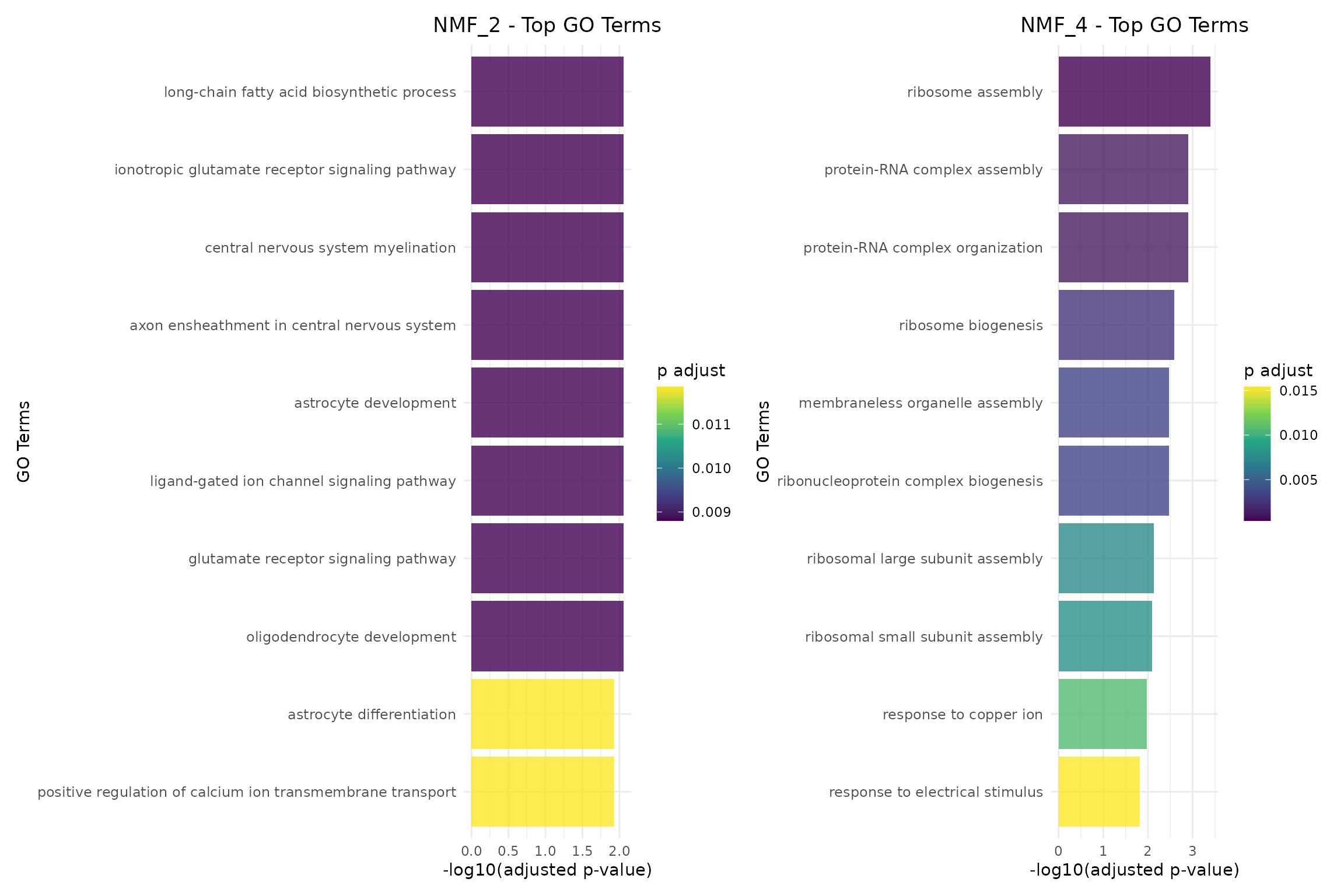
Bar Charts
Bar charts show the most significantly enriched terms with clear ranking:
# Create bar charts for the first two programs
if (length(go_results) >= 2) {
  program1_name <- names(go_results)[1]
  program2_name <- names(go_results)[2]

  p1 <- plotGOBarChart(go_results[[program1_name]],
                      n_terms = 10,
                      title = paste(program1_name, "- Top GO Terms"))

  p2 <- plotGOBarChart(go_results[[program2_name]],
                      n_terms = 10,
                      title = paste(program2_name, "- Top GO Terms"))

  # Show side by side
  p1 + p2
} else if (length(go_results) == 1) {
  plotGOBarChart(go_results[[1]], n_terms = 12,
                title = paste(names(go_results)[1], "- GO Enrichment"))
}
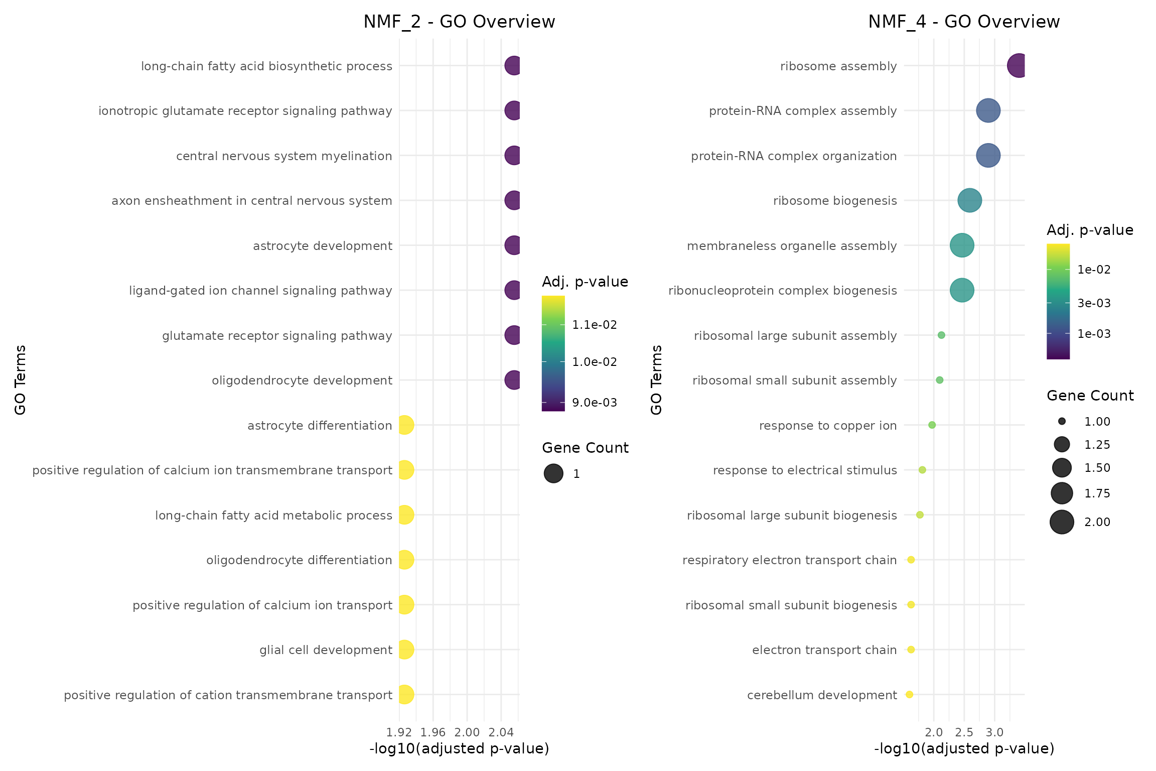
Dot Plots
Dot plots encode both significance and gene count information:
# Create dot plots with size representing gene count
if (length(go_results) >= 2) {
  p1_dot <- plotGODotPlot(go_results[[program1_name]],
                         n_terms = 15,
                         title = paste(program1_name, "- GO Overview"))

  p2_dot <- plotGODotPlot(go_results[[program2_name]],
                         n_terms = 15,
                         title = paste(program2_name, "- GO Overview"))

  p1_dot + p2_dot
} else if (length(go_results) == 1) {
  plotGODotPlot(go_results[[1]], n_terms = 15,
               title = paste(names(go_results)[1], "- GO Overview"))
}
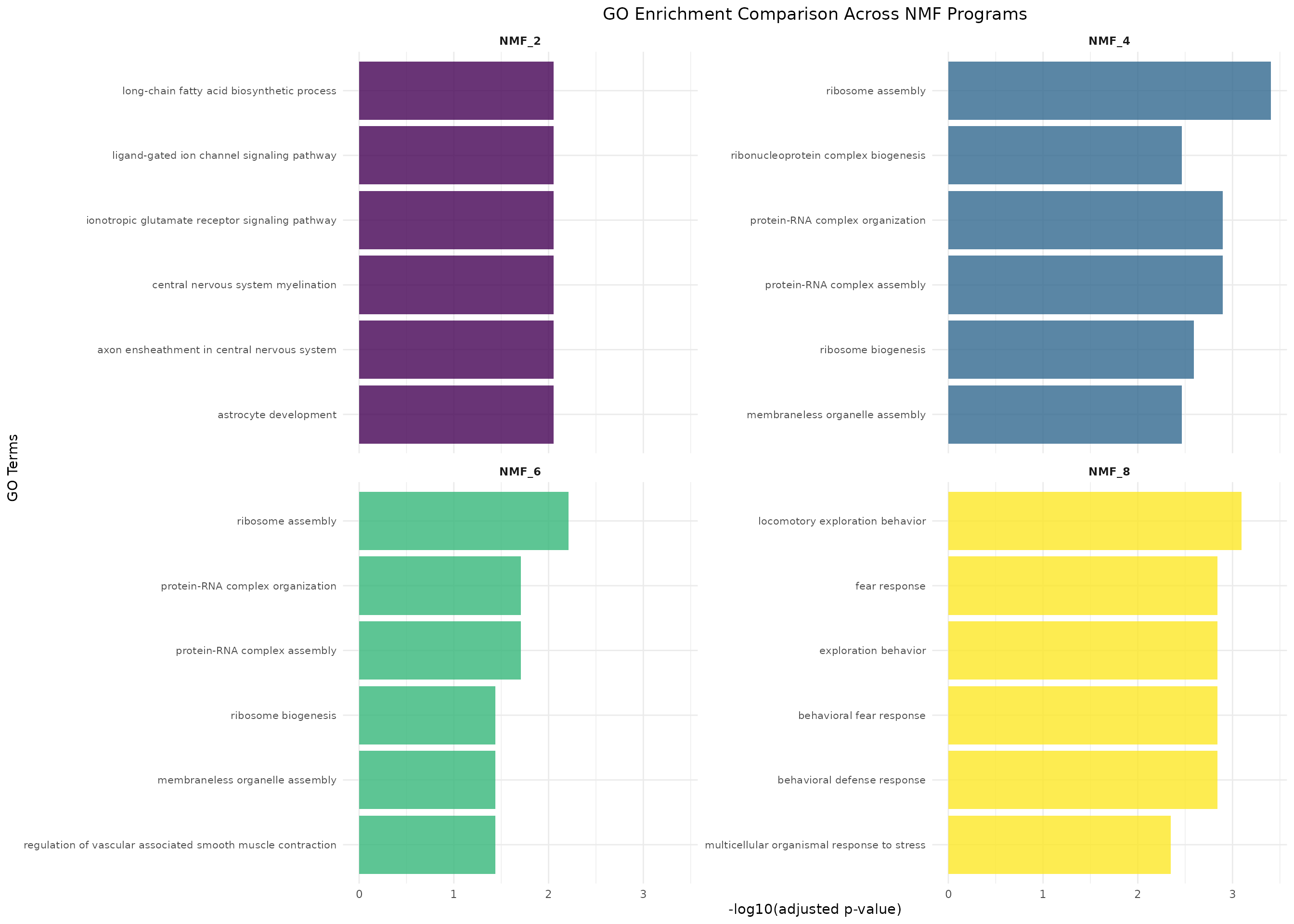
Multi-Program Comparison
Compare GO terms across all programs to identify program-specific functions:
# Multi-program comparison
if (length(go_results) > 1) {
  comparison_plot <- plotMultipleProgramsGO(go_results,
                                           n_terms = 6,  # Top 6 terms per program
                                           ncol = 2)     # 2 columns layout
  comparison_plot
}
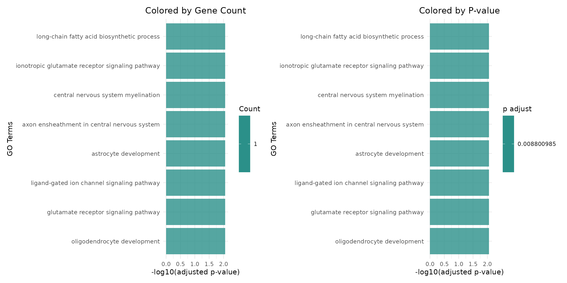
Alternative Visualizations
Different Color Schemes
if (length(go_results) >= 1) {
  program_name <- names(go_results)[1]

  # Color by gene count instead of p-value
  p_count <- plotGOBarChart(go_results[[program_name]],
                           n_terms = 8,
                           color_by = "Count",
                           title = "Colored by Gene Count")

  # Standard p-value coloring
  p_pval <- plotGOBarChart(go_results[[program_name]],
                          n_terms = 8,
                          color_by = "p.adjust",
                          title = "Colored by P-value")

  p_count + p_pval
}
Biological Interpretation
The GO enrichment results reveal the biological functions of each NMF program:
Brain-Specific Patterns
Let’s look for brain-specific GO terms and markers in our results:
# Look for brain-related GO terms
brain_keywords <- c("neuron", "axon", "dendrite", "synapse", "myelination",
                   "oligodendrocyte", "astrocyte", "microglia", "neural")

# Search for brain-related terms in each program
for (i in seq_along(go_results)) {
  program_name <- names(go_results)[i]
  go_result <- go_results[[program_name]]

  if (nrow(go_result) > 0) {
    # Convert to data.frame if needed
    if (inherits(go_result, "enrichResult")) {
      go_df <- as.data.frame(go_result)
    } else {
      go_df <- go_result
    }

    # Find brain-related terms
    brain_terms <- go_df[grepl(paste(brain_keywords, collapse = "|"),
                              go_df$Description, ignore.case = TRUE), ]

    if (nrow(brain_terms) > 0) {
      cat("\n=== Brain-related GO terms in", program_name, "===\n")
      cat("Found", nrow(brain_terms), "brain-related terms:\n")
      print(head(brain_terms[, c("Description", "p.adjust", "Count")], 4))
    }
  }
}
#>
#> === Brain-related GO terms in NMF_2 ===
#> Found 9 brain-related terms:
#>                                            Description    p.adjust Count
#> GO:0022010          central nervous system myelination 0.008800985     1
#> GO:0032291 axon ensheathment in central nervous system 0.008800985     1
#> GO:0014002                       astrocyte development 0.008800985     1
#> GO:0014003                 oligodendrocyte development 0.008800985     1
#>
#> === Brain-related GO terms in NMF_8 ===
#> Found 19 brain-related terms:
#>                                            Description   p.adjust Count
#> GO:0019227       neuronal action potential propagation 0.01441277     1
#> GO:1905809 negative regulation of synapse organization 0.01443348     1
#> GO:0045773       positive regulation of axon extension 0.01686036     1
#> GO:0050772         positive regulation of axonogenesis 0.02199347     1
Program Characterization
Based on the top genes and GO terms, we can characterize each program:
# Get top genes for each program to aid interpretation
top_genes_list <- getTopFeatures(sce, n = 10)

for (i in 1:min(4, length(top_genes_list))) {
  program_name <- names(top_genes_list)[i]
  cat("\n=== Program", i, "Characterization ===\n")
  cat("Top genes:", paste(head(top_genes_list[[program_name]], 8), collapse = ", "), "\n")

  # Show top GO term
  if (program_name %in% names(go_results)) {
    go_result <- go_results[[program_name]]
    if (nrow(go_result) > 0) {
      if (inherits(go_result, "enrichResult")) {
        top_go <- as.data.frame(go_result)[1, "Description"]
      } else {
        top_go <- go_result[1, "Description"]
      }
      cat("Top GO term:", top_go, "\n")
    }
  }
}
#>
#> === Program 1 Characterization ===
#> Top genes: Ppp3ca, Calm2, Atp1b1, Hpca, Cpe, Tspan13, Rtn1, Atp2b1
#>
#> === Program 2 Characterization ===
#> Top genes: Plp1, Trf, Mal, Mog, Mbp, Apod, Cnp, Ugt8a
#> Top GO term: long-chain fatty acid biosynthetic process
#>
#> === Program 3 Characterization ===
#> Top genes: Nrgn, Mef2c, Snap25, Rtn1, Camk2n1, Atp1b1, Basp1, Calm2
#>
#> === Program 4 Characterization ===
#> Top genes: mt-Rnr2, mt-Co1, mt-Rnr1, Tmsb4x, Usmg5, Mdh1, Zwint, Calm2
#> Top GO term: ribosome assembly
Saving Results
# Save comprehensive plots to PDF
saveGOPlotsToPDF(go_results,
                filename = "brain_nmf_go_enrichment.pdf",
                width = 14, height = 10)
#> Creating plots for NMF_2
#> Creating plots for NMF_4
#> Creating plots for NMF_6
#> Creating plots for NMF_8
#> Creating comparison plot
#> GO plots saved to brain_nmf_go_enrichment.pdf

# Save results for later analysis
save(go_results, sce, file = "brain_nmf_enrichment_analysis.RData")

cat("Results saved to brain_nmf_go_enrichment.pdf and brain_nmf_enrichment_analysis.RData\n")
#> Results saved to brain_nmf_go_enrichment.pdf and brain_nmf_enrichment_analysis.RData
Advanced Analysis
Custom Gene Sets
You can also perform enrichment with custom gene sets:
# Example: Create custom brain cell type markers (not run)
custom_gene_sets <- list(
  "Oligodendrocyte_markers" = c("Mbp", "Plp1", "Mog", "Cnp"),
  "Astrocyte_markers" = c("Gfap", "Aldh1l1", "Aqp4", "Slc1a3"),
  "Neuron_markers" = c("Rbfox3", "Tubb3", "Map2", "Syn1")
)

# Use prepareProgramGeneSets to create gene sets for enrichment
program_gene_sets <- prepareProgramGeneSets(sce, n_genes = 30)
Network Visualization
For programs with many GO terms, network plots can show term relationships:
# Network visualization (requires enrichplot package)
if (requireNamespace("enrichplot", quietly = TRUE) && length(go_results) > 0) {
  # This works best with full enrichResult objects
  program_with_most_terms <- which.max(sapply(go_results, nrow))
  if (inherits(go_results[[program_with_most_terms]], "enrichResult")) {
    network_plot <- plotGONetwork(go_results[[program_with_most_terms]],
                                 n_terms = 20,
                                 title = "GO Terms Network")
    print(network_plot)
  }
}
Summary
This vignette demonstrated:
- NMF analysis of brain single-cell data to identify gene expression programs
- GO enrichment analysis to understand program functions
- Multiple visualization approaches for enrichment results
- Biological interpretation of brain cell type programs
- Comparison across programs to identify specific functions
Key Takeaways
- NMF programs often correspond to cell type-specific expression signatures
- GO enrichment helps validate and interpret these programs biologically
- Different visualization approaches highlight different aspects of enrichment
- Multi-program comparisons reveal program-specific vs shared functions
Next Steps
- Explore other ontologies (MF, CC) and pathway databases (KEGG, Reactome)
- Compare enrichment across different experimental conditions
- Integrate with trajectory analysis or pseudotime
- Perform cross-species comparisons of program functions
sessionInfo()
#> R version 4.5.1 (2025-06-13)
#> Platform: x86_64-pc-linux-gnu
#> Running under: Ubuntu 24.04.3 LTS
#>
#> Matrix products: default
#> BLAS:   /usr/lib/x86_64-linux-gnu/openblas-pthread/libblas.so.3
#> LAPACK: /usr/lib/x86_64-linux-gnu/openblas-pthread/libopenblasp-r0.3.26.so;  LAPACK version 3.12.0
#>
#> locale:
#>  [1] LC_CTYPE=C.UTF-8       LC_NUMERIC=C           LC_TIME=C.UTF-8
#>  [4] LC_COLLATE=C.UTF-8     LC_MONETARY=C.UTF-8    LC_MESSAGES=C.UTF-8
#>  [7] LC_PAPER=C.UTF-8       LC_NAME=C              LC_ADDRESS=C
#> [10] LC_TELEPHONE=C         LC_MEASUREMENT=C.UTF-8 LC_IDENTIFICATION=C
#>
#> time zone: UTC
#> tzcode source: system (glibc)
#>
#> attached base packages:
#> [1] stats4    stats     graphics  grDevices utils     datasets  methods
#> [8] base
#>
#> other attached packages:
#>  [1] Matrix_1.7-3                org.Mm.eg.db_3.21.0
#>  [3] AnnotationDbi_1.70.0        clusterProfiler_4.16.0
#>  [5] patchwork_1.3.2             scran_1.36.0
#>  [7] scater_1.36.0               ggplot2_4.0.0
#>  [9] scuttle_1.18.0              scRNAseq_2.22.0
#> [11] NMFscape_0.99.0             SingleCellExperiment_1.30.1
#> [13] SummarizedExperiment_1.38.1 Biobase_2.68.0
#> [15] GenomicRanges_1.60.0        GenomeInfoDb_1.44.2
#> [17] IRanges_2.42.0              S4Vectors_0.46.0
#> [19] MatrixGenerics_1.20.0       matrixStats_1.5.0
#> [21] BiocGenerics_0.54.0         generics_0.1.4
#> [23] BiocStyle_2.36.0
#>
#> loaded via a namespace (and not attached):
#>   [1] splines_4.5.1            BiocIO_1.18.0            ggplotify_0.1.2
#>   [4] bitops_1.0-9             filelock_1.0.3           tibble_3.3.0
#>   [7] R.oo_1.27.1              XML_3.99-0.19            lifecycle_1.0.4
#>  [10] httr2_1.2.1              edgeR_4.6.3              lattice_0.22-7
#>  [13] ensembldb_2.32.0         alabaster.base_1.8.1     magrittr_2.0.3
#>  [16] limma_3.64.3             sass_0.4.10              rmarkdown_2.29
#>  [19] jquerylib_0.1.4          yaml_2.3.10              ggtangle_0.0.7
#>  [22] metapod_1.16.0           cowplot_1.2.0            DBI_1.2.3
#>  [25] RColorBrewer_1.1-3       abind_1.4-8              purrr_1.1.0
#>  [28] R.utils_2.13.0           AnnotationFilter_1.32.0  RCurl_1.98-1.17
#>  [31] yulab.utils_0.2.1        rappdirs_0.3.3           GenomeInfoDbData_1.2.14
#>  [34] enrichplot_1.28.4        ggrepel_0.9.6            irlba_2.3.5.1
#>  [37] alabaster.sce_1.8.0      tidytree_0.4.6           pheatmap_1.0.13
#>  [40] dqrng_0.4.1              pkgdown_2.1.3            codetools_0.2-20
#>  [43] DelayedArray_0.34.1      DOSE_4.2.0               tidyselect_1.2.1
#>  [46] aplot_0.2.8              UCSC.utils_1.4.0         farver_2.1.2
#>  [49] ScaledMatrix_1.16.0      viridis_0.6.5            BiocFileCache_2.16.2
#>  [52] GenomicAlignments_1.44.0 jsonlite_2.0.0           BiocNeighbors_2.2.0
#>  [55] systemfonts_1.2.3        tools_4.5.1              treeio_1.32.0
#>  [58] ragg_1.5.0               Rcpp_1.1.0               glue_1.8.0
#>  [61] gridExtra_2.3            SparseArray_1.8.1        xfun_0.53
#>  [64] qvalue_2.40.0            dplyr_1.1.4              HDF5Array_1.36.0
#>  [67] gypsum_1.4.0             withr_3.0.2              BiocManager_1.30.26
#>  [70] fastmap_1.2.0            rhdf5filters_1.20.0      bluster_1.18.0
#>  [73] RcppML_0.3.7             digest_0.6.37            rsvd_1.0.5
#>  [76] gridGraphics_0.5-1       R6_2.6.1                 textshaping_1.0.3
#>  [79] GO.db_3.21.0             RSQLite_2.4.3            R.methodsS3_1.8.2
#>  [82] h5mread_1.0.1            tidyr_1.3.1              data.table_1.17.8
#>  [85] FNN_1.1.4.1              rtracklayer_1.68.0       httr_1.4.7
#>  [88] S4Arrays_1.8.1           uwot_0.2.3               pkgconfig_2.0.3
#>  [91] gtable_0.3.6             blob_1.2.4               S7_0.2.0
#>  [94] XVector_0.48.0           htmltools_0.5.8.1        fgsea_1.34.2
#>  [97] bookdown_0.44            ProtGenerics_1.40.0      scales_1.4.0
#> [100] alabaster.matrix_1.8.0   png_0.1-8                ggfun_0.2.0
#> [103] knitr_1.50               reshape2_1.4.4           rjson_0.2.23
#> [106] nlme_3.1-168             curl_7.0.0               cachem_1.1.0
#> [109] rhdf5_2.52.1             stringr_1.5.2            BiocVersion_3.21.1
#> [112] parallel_4.5.1           vipor_0.4.7              restfulr_0.0.16
#> [115] desc_1.4.3               pillar_1.11.0            grid_4.5.1
#> [118] alabaster.schemas_1.8.0  vctrs_0.6.5              BiocSingular_1.24.0
#> [121] dbplyr_2.5.1             beachmat_2.24.0          cluster_2.1.8.1
#> [124] beeswarm_0.4.0           evaluate_1.0.5           GenomicFeatures_1.60.0
#> [127] cli_3.6.5                locfit_1.5-9.12          compiler_4.5.1
#> [130] Rsamtools_2.24.1         rlang_1.1.6              crayon_1.5.3
#> [133] labeling_0.4.3           plyr_1.8.9               fs_1.6.6
#> [136] ggbeeswarm_0.7.2         stringi_1.8.7            alabaster.se_1.8.0
#> [139] viridisLite_0.4.2        BiocParallel_1.42.1      Biostrings_2.76.0
#> [142] lazyeval_0.2.2           GOSemSim_2.34.0          ExperimentHub_2.16.1
#> [145] bit64_4.6.0-1            Rhdf5lib_1.30.0          KEGGREST_1.48.1
#> [148] statmod_1.5.0            alabaster.ranges_1.8.0   AnnotationHub_3.16.1
#> [151] igraph_2.1.4             memoise_2.0.1            bslib_0.9.0
#> [154] ggtree_3.16.3            fastmatch_1.1-6          bit_4.6.0
#> [157] gson_0.1.0               ape_5.8-1