Getting Started with NMFscape
Michael Totty
2025-09-12
Source:vignettes/getting-started.Rmd
getting-started.RmdIntroduction
NMFscape provides fast, scalable non-negative matrix factorization (NMF) for single-cell and spatial genomics data. NMF decomposes gene expression data into biologically interpretable gene expression programs and their usage patterns across cells.
Why NMF?
- Biologically interpretable: Gene programs contain only positive weights
-
Parts-based decomposition: Identifies co-expressed
gene modules
- Cell type discovery: Programs often correspond to cell type signatures
- Additive mixing: Cells can express multiple programs simultaneously
NMFscape uses RcppML for high-performance computation and integrates seamlessly with Bioconductor workflows.
library(NMFscape)
#> Loading required package: BiocGenerics
#> Loading required package: generics
#>
#> Attaching package: 'generics'
#> The following objects are masked from 'package:base':
#>
#>     as.difftime, as.factor, as.ordered, intersect, is.element, setdiff,
#>     setequal, union
#>
#> Attaching package: 'BiocGenerics'
#> The following objects are masked from 'package:stats':
#>
#>     IQR, mad, sd, var, xtabs
#> The following objects are masked from 'package:base':
#>
#>     anyDuplicated, aperm, append, as.data.frame, basename, cbind,
#>     colnames, dirname, do.call, duplicated, eval, evalq, Filter, Find,
#>     get, grep, grepl, is.unsorted, lapply, Map, mapply, match, mget,
#>     order, paste, pmax, pmax.int, pmin, pmin.int, Position, rank,
#>     rbind, Reduce, rownames, sapply, saveRDS, table, tapply, unique,
#>     unsplit, which.max, which.min
#> Loading required package: SingleCellExperiment
#> Loading required package: SummarizedExperiment
#> Loading required package: MatrixGenerics
#> Loading required package: matrixStats
#>
#> Attaching package: 'MatrixGenerics'
#> The following objects are masked from 'package:matrixStats':
#>
#>     colAlls, colAnyNAs, colAnys, colAvgsPerRowSet, colCollapse,
#>     colCounts, colCummaxs, colCummins, colCumprods, colCumsums,
#>     colDiffs, colIQRDiffs, colIQRs, colLogSumExps, colMadDiffs,
#>     colMads, colMaxs, colMeans2, colMedians, colMins, colOrderStats,
#>     colProds, colQuantiles, colRanges, colRanks, colSdDiffs, colSds,
#>     colSums2, colTabulates, colVarDiffs, colVars, colWeightedMads,
#>     colWeightedMeans, colWeightedMedians, colWeightedSds,
#>     colWeightedVars, rowAlls, rowAnyNAs, rowAnys, rowAvgsPerColSet,
#>     rowCollapse, rowCounts, rowCummaxs, rowCummins, rowCumprods,
#>     rowCumsums, rowDiffs, rowIQRDiffs, rowIQRs, rowLogSumExps,
#>     rowMadDiffs, rowMads, rowMaxs, rowMeans2, rowMedians, rowMins,
#>     rowOrderStats, rowProds, rowQuantiles, rowRanges, rowRanks,
#>     rowSdDiffs, rowSds, rowSums2, rowTabulates, rowVarDiffs, rowVars,
#>     rowWeightedMads, rowWeightedMeans, rowWeightedMedians,
#>     rowWeightedSds, rowWeightedVars
#> Loading required package: GenomicRanges
#> Loading required package: stats4
#> Loading required package: S4Vectors
#>
#> Attaching package: 'S4Vectors'
#> The following object is masked from 'package:utils':
#>
#>     findMatches
#> The following objects are masked from 'package:base':
#>
#>     expand.grid, I, unname
#> Loading required package: IRanges
#> Loading required package: GenomeInfoDb
#> Loading required package: Biobase
#> Welcome to Bioconductor
#>
#>     Vignettes contain introductory material; view with
#>     'browseVignettes()'. To cite Bioconductor, see
#>     'citation("Biobase")', and for packages 'citation("pkgname")'.
#>
#> Attaching package: 'Biobase'
#> The following object is masked from 'package:MatrixGenerics':
#>
#>     rowMedians
#> The following objects are masked from 'package:matrixStats':
#>
#>     anyMissing, rowMedians
#> Warning: replacing previous import 'BiocGenerics::sd' by 'stats::sd' when
#> loading 'NMFscape'
library(SingleCellExperiment)
library(scuttle)
library(scater)
#> Loading required package: ggplot2
library(scran)
library(scRNAseq)
library(ggplot2)
library(patchwork)
Basic NMF Workflow
Load and prepare data
We’ll use the Zeisel brain dataset (Zeisel et al. 2015, Science) which contains diverse brain cell types.
# Load brain dataset
sce <- ZeiselBrainData()
cat("Original data:", nrow(sce), "genes,", ncol(sce), "cells\n")
#> Original data: 20006 genes, 3005 cells

# Quality control and filtering
sce <- addPerCellQCMetrics(sce)
sce <- addPerFeatureQCMetrics(sce)
sce <- sce[rowData(sce)$detected >= 10, ]  # Genes detected in ≥10 cells
sce <- sce[, colData(sce)$detected >= 500]  # Cells with ≥500 detected genes

# Subset to 1000 cells for computational efficiency
set.seed(42)
if (ncol(sce) > 1000) {
  cell_subset <- sample(ncol(sce), 1000)
  sce <- sce[, cell_subset]
}

# Normalize and select highly variable genes
sce <- logNormCounts(sce)
dec <- modelGeneVar(sce)
top_hvgs <- getTopHVGs(dec, n = 1000)  # Top 1000 HVGs
sce <- sce[top_hvgs, ]

cat("Final data:", nrow(sce), "genes,", ncol(sce), "cells\n")
#> Final data: 1000 genes, 1000 cells
Run NMF
# Run NMF with 8 programs (good for brain cell diversity)
sce <- runNMFscape(sce, k = 8, verbose = FALSE)
#>
#> Attaching package: 'Matrix'
#> The following object is masked from 'package:S4Vectors':
#>
#>     expand

# Check results
cat("NMF programs stored in:", reducedDimNames(sce), "\n")
#> NMF programs stored in: NMF
cat("Basis matrix stored in:", names(metadata(sce)), "\n")
#> Basis matrix stored in: NMF_basis
Add dimension reductions for visualization
# Run PCA and UMAP for visualization
sce <- runPCA(sce, ncomponents = 50)
sce <- runUMAP(sce, dimred = "PCA")

cat("Available dimension reductions:", reducedDimNames(sce), "\n")
#> Available dimension reductions: NMF PCA UMAP
Visualizing NMF Results
Plot NMF programs on UMAP
NMFscape provides convenient visualization functions to plot NMF program usage on dimension reduction coordinates.
# Visualize two distinct NMF programs
p1 <- vizUMAP(sce, program = 1, title = "NMF Program 1")
p2 <- vizUMAP(sce, program = 3, title = "NMF Program 3", color_scale = "plasma")

# Display side by side
p1 + p2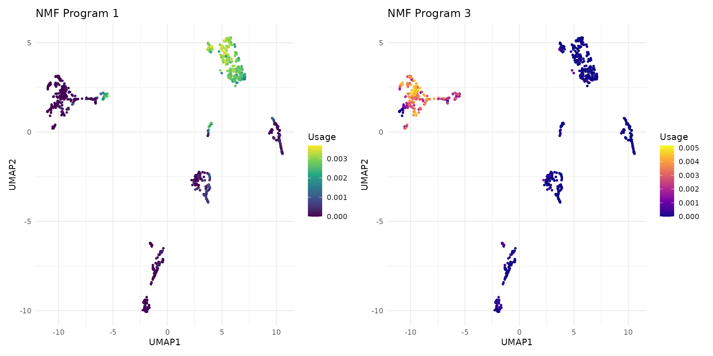
# Compare with known cell types
p3 <- plotReducedDim(sce, dimred = "UMAP", colour_by = "level1class",
                     point_size = 0.8) +
  ggtitle("Known Cell Types") +
  theme(legend.position = "right")

# Show NMF programs vs cell types
(p1 + p2) / p3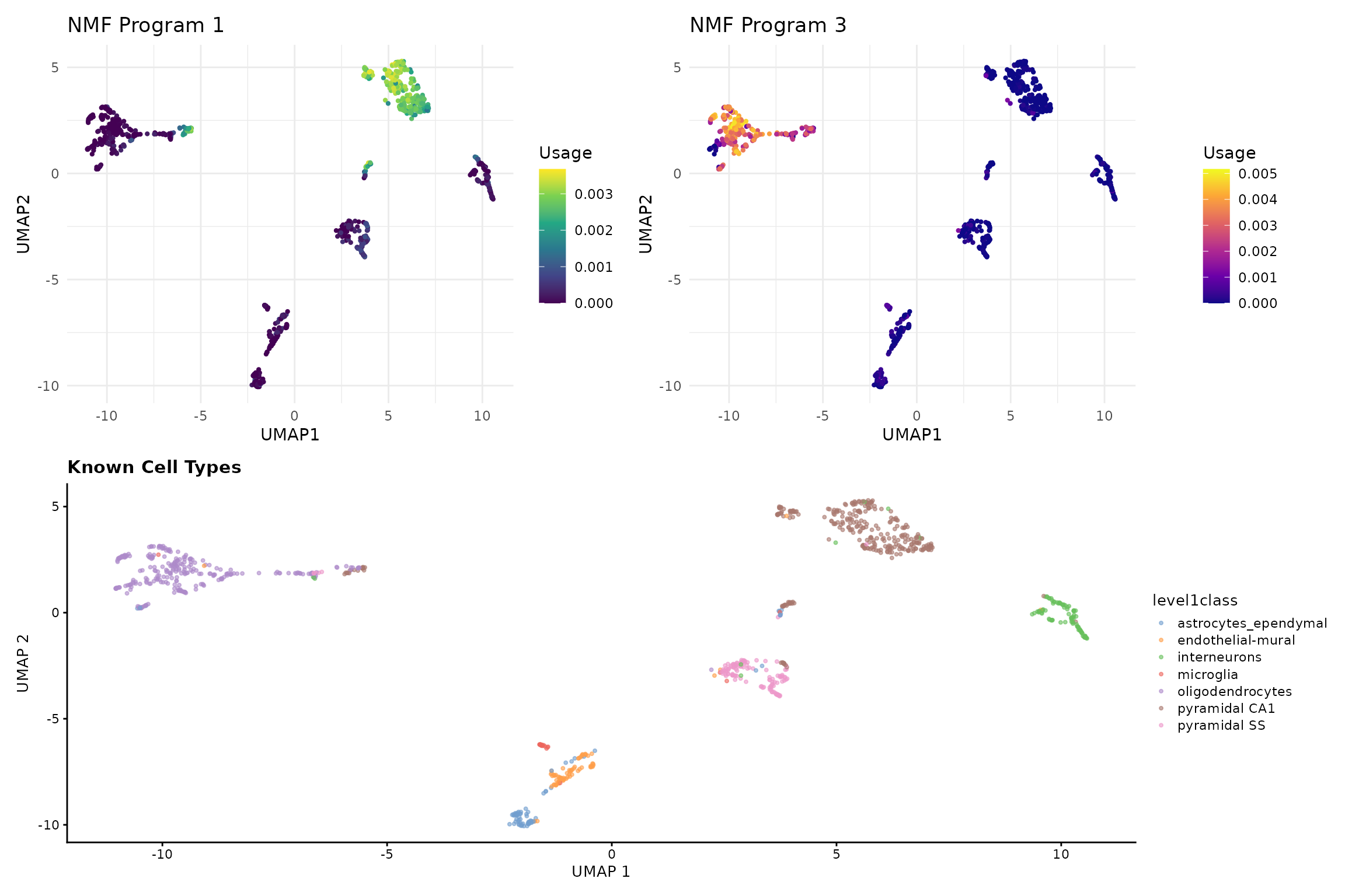
Examine top genes per program
# Get top contributing genes for each program
top_genes <- getTopFeatures(sce, n = 10)

# Display top genes for first few programs
for (i in 1:4) {
  cat("Program", i, "top genes:", paste(top_genes[[i]][1:5], collapse = ", "), "...\n")
}
#> Program 1 top genes: Atp2b1, Meg3, Gria2, Ppp3ca, Atp1b1 ...
#> Program 2 top genes: Usmg5, Mdh1, Calm2, Cycs, Atpif1 ...
#> Program 3 top genes: Plp1, Trf, Apod, Mal, Car2 ...
#> Program 4 top genes: Meg3, Nrgn, Arpp21, Mef2c, Atp2b1 ...
Key Functions
-
runNMFscape(): Run NMF decomposition -
getBasis(): Extract gene expression programs (genes × programs) -
getCoefficients(): Extract program usage (cells × programs)
-
getTopFeatures(): Get top genes per program -
vizUMAP(): Visualize programs on UMAP coordinates -
vizDimRed(): Visualize programs on any dimension reduction
Session Information
sessionInfo()
#> R version 4.5.1 (2025-06-13)
#> Platform: x86_64-pc-linux-gnu
#> Running under: Ubuntu 24.04.3 LTS
#>
#> Matrix products: default
#> BLAS:   /usr/lib/x86_64-linux-gnu/openblas-pthread/libblas.so.3
#> LAPACK: /usr/lib/x86_64-linux-gnu/openblas-pthread/libopenblasp-r0.3.26.so;  LAPACK version 3.12.0
#>
#> locale:
#>  [1] LC_CTYPE=C.UTF-8       LC_NUMERIC=C           LC_TIME=C.UTF-8
#>  [4] LC_COLLATE=C.UTF-8     LC_MONETARY=C.UTF-8    LC_MESSAGES=C.UTF-8
#>  [7] LC_PAPER=C.UTF-8       LC_NAME=C              LC_ADDRESS=C
#> [10] LC_TELEPHONE=C         LC_MEASUREMENT=C.UTF-8 LC_IDENTIFICATION=C
#>
#> time zone: UTC
#> tzcode source: system (glibc)
#>
#> attached base packages:
#> [1] stats4    stats     graphics  grDevices utils     datasets  methods
#> [8] base
#>
#> other attached packages:
#>  [1] Matrix_1.7-3                patchwork_1.3.2
#>  [3] scRNAseq_2.22.0             scran_1.36.0
#>  [5] scater_1.36.0               ggplot2_4.0.0
#>  [7] scuttle_1.18.0              NMFscape_0.99.0
#>  [9] SingleCellExperiment_1.30.1 SummarizedExperiment_1.38.1
#> [11] Biobase_2.68.0              GenomicRanges_1.60.0
#> [13] GenomeInfoDb_1.44.2         IRanges_2.42.0
#> [15] S4Vectors_0.46.0            MatrixGenerics_1.20.0
#> [17] matrixStats_1.5.0           BiocGenerics_0.54.0
#> [19] generics_0.1.4              BiocStyle_2.36.0
#>
#> loaded via a namespace (and not attached):
#>   [1] RColorBrewer_1.1-3       jsonlite_2.0.0           magrittr_2.0.3
#>   [4] gypsum_1.4.0             ggbeeswarm_0.7.2         GenomicFeatures_1.60.0
#>   [7] farver_2.1.2             rmarkdown_2.29           BiocIO_1.18.0
#>  [10] fs_1.6.6                 ragg_1.5.0               vctrs_0.6.5
#>  [13] Rsamtools_2.24.1         memoise_2.0.1            RCurl_1.98-1.17
#>  [16] htmltools_0.5.8.1        S4Arrays_1.8.1           AnnotationHub_3.16.1
#>  [19] curl_7.0.0               BiocNeighbors_2.2.0      Rhdf5lib_1.30.0
#>  [22] rhdf5_2.52.1             SparseArray_1.8.1        alabaster.base_1.8.1
#>  [25] sass_0.4.10              bslib_0.9.0              alabaster.sce_1.8.0
#>  [28] desc_1.4.3               httr2_1.2.1              cachem_1.1.0
#>  [31] GenomicAlignments_1.44.0 igraph_2.1.4             lifecycle_1.0.4
#>  [34] pkgconfig_2.0.3          rsvd_1.0.5               R6_2.6.1
#>  [37] fastmap_1.2.0            GenomeInfoDbData_1.2.14  digest_0.6.37
#>  [40] AnnotationDbi_1.70.0     dqrng_0.4.1              irlba_2.3.5.1
#>  [43] ExperimentHub_2.16.1     textshaping_1.0.3        RSQLite_2.4.3
#>  [46] beachmat_2.24.0          labeling_0.4.3           filelock_1.0.3
#>  [49] httr_1.4.7               abind_1.4-8              compiler_4.5.1
#>  [52] bit64_4.6.0-1            withr_3.0.2              S7_0.2.0
#>  [55] BiocParallel_1.42.1      viridis_0.6.5            DBI_1.2.3
#>  [58] alabaster.ranges_1.8.0   HDF5Array_1.36.0         alabaster.schemas_1.8.0
#>  [61] rappdirs_0.3.3           DelayedArray_0.34.1      rjson_0.2.23
#>  [64] bluster_1.18.0           tools_4.5.1              vipor_0.4.7
#>  [67] beeswarm_0.4.0           glue_1.8.0               h5mread_1.0.1
#>  [70] restfulr_0.0.16          rhdf5filters_1.20.0      grid_4.5.1
#>  [73] cluster_2.1.8.1          gtable_0.3.6             ensembldb_2.32.0
#>  [76] RcppML_0.3.7             BiocSingular_1.24.0      ScaledMatrix_1.16.0
#>  [79] metapod_1.16.0           XVector_0.48.0           ggrepel_0.9.6
#>  [82] BiocVersion_3.21.1       pillar_1.11.0            limma_3.64.3
#>  [85] dplyr_1.1.4              BiocFileCache_2.16.2     lattice_0.22-7
#>  [88] FNN_1.1.4.1              rtracklayer_1.68.0       bit_4.6.0
#>  [91] tidyselect_1.2.1         locfit_1.5-9.12          Biostrings_2.76.0
#>  [94] knitr_1.50               gridExtra_2.3            bookdown_0.44
#>  [97] ProtGenerics_1.40.0      edgeR_4.6.3              xfun_0.53
#> [100] statmod_1.5.0            pheatmap_1.0.13          UCSC.utils_1.4.0
#> [103] lazyeval_0.2.2           yaml_2.3.10              evaluate_1.0.5
#> [106] codetools_0.2-20         tibble_3.3.0             alabaster.matrix_1.8.0
#> [109] BiocManager_1.30.26      cli_3.6.5                uwot_0.2.3
#> [112] systemfonts_1.2.3        jquerylib_0.1.4          Rcpp_1.1.0
#> [115] dbplyr_2.5.1             png_0.1-8                XML_3.99-0.19
#> [118] parallel_4.5.1           pkgdown_2.1.3            blob_1.2.4
#> [121] AnnotationFilter_1.32.0  bitops_1.0-9             alabaster.se_1.8.0
#> [124] viridisLite_0.4.2        scales_1.4.0             crayon_1.5.3
#> [127] rlang_1.1.6              cowplot_1.2.0            KEGGREST_1.48.1